

Reasoning Under Uncertainty: The Decision Layer of a Cross-Chain MEV Bot
How a searcher decides whether to trade, how much, and at what risk
The simulation layer tells you the deterministic PnL of a route: given this pool state, this input size, and this AMM math, the output is X. That number is correct.
It is also insufficient to make a trading decision.
A cross-chain arbitrage is not a deterministic event. Between the moment you observe an opportunity and the moment it either executes or does not, several things can go wrong independently:
Your transaction may not be included in the target block.
If it is included, the bridge message may fail or arrive late.
By the time the second leg executes on the destination chain, the price may have moved enough to eliminate the profit.
A competing searcher may have already closed the gap.
Your infrastructure: RPC, indexer, bundle relay, may introduce enough latency to make the market state you simulated stale.
Each of these is a separate random variable. The decision layer is the component that reasons about all of them together, translates the deterministic PnL into a probability-weighted expected value, and then allocates capital across multiple opportunities at the same block without double-counting risk or over-committing to a single route.
Without this layer, you are reading an accurate number and then guessing what to do with it.
Expected value as the decision unit
Expected value is the probability-weighted average outcome of a trade. If an arbitrage has a deterministic PnL of $100 but only executes successfully 60% of the time and causes a $30 loss the other 40%, its EV is not $100, it is:
0.6 × $100 − 0.4 × $30 = $48.
This matters for two reasons. First, it lets you compare opportunities with very different risk profiles on a common scale: a low-probability high-profit route and a high-probability low-profit route are only comparable once you weight their outcomes by likelihood. Second, it is the correct objective for capital allocation , deploying capital where EV per unit is highest maximises long-run returns, even when individual trades fail.
Optimising for deterministic PnL alone ignores execution risk entirely. Optimising for success probability alone ignores the magnitude of outcomes.
EV combines both, and it is the number every component in the decision layer is ultimately trying to maximise. The rest of this article is about how it is computed.
The three-phase pipeline
Every tick , whether driven by a live node or a historical block snapshot , runs the same three-phase pipeline:
discoverCandidateBundles() → route discovery + profit-only sizingsimulateBundles() → EV(r, s) for each route × size pointcapitalAllocator.allocate() → greedy marginal assignment of available capital
The entry point is BundleDecisionFlow, which exposes two methods: onChainTick() for the live bot and fromDatabase() for the backtester. Both call the same internal processState(). The decision logic does not know or care whether the market state came from a live node or a database snapshot , the pipeline is identical in both modes. This is intentional: the backtester must reproduce exactly what the live bot would have done, not an approximation of it.
Phase 1 , Discovery identifies candidate bundles from the current market state. Routes are screened for profitability, then grouped into non-conflicting bundles , sets of routes that do not share any pool and can therefore be simulated together without state cross-contamination.
Phase 2 , Simulation runs BundleSimulationEngine over each candidate bundle. For every route and every point in the size grid around sStar, EvEstimator computes the full probabilistic EV and tail risk. This phase is capital-agnostic: it does not know what capital is available, it just produces the EV(size) curve for every route.
Phase 3 , Allocation runs CapitalAllocator over the simulation results. It takes the EV(size) curves, derives marginal increments across all routes, and greedily assigns available capital to the highest-marginal-return increments first. The output is an AllocatedBundle: the final set of routes with their assigned sizes and the adjusted total EV after capital constraints.

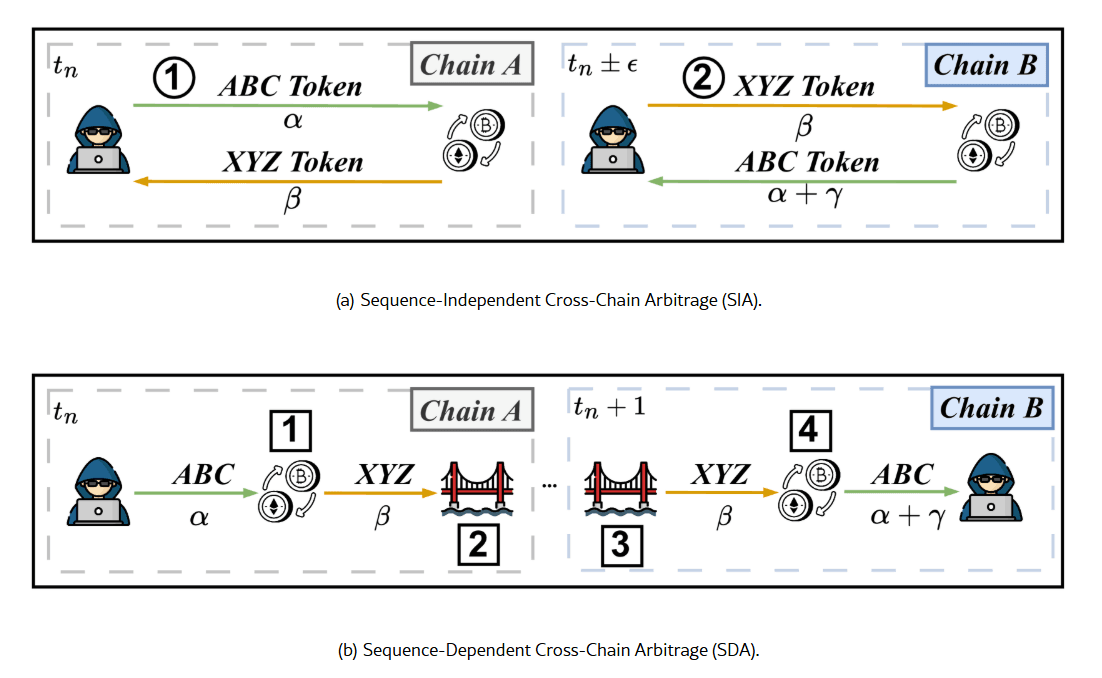
SIA vs SDA , two different games
Not all cross-chain arbitrage routes have the same structure. The decision layer models two distinct types, because the risk profile of each is fundamentally different.

SIA , Sequence-Independent Arbitrage. Both legs are submitted together and the order of execution does not matter , neither leg depends on the other completing first. A key structural requirement is inventory: the searcher must hold the required assets on both chains before submitting, since there is no bridge step to transfer capital between legs. The capital is pre-positioned, and the trade works only if sufficient inventory exists on each chain at execution time.
SDA , Sequence-Dependent Arbitrage. Leg A executes first on the origin chain. The asset is then transferred across chains via a bridge. Leg B executes on the destination chain after the bridge settles. The dominant risk here is not pre-execution price movement but inventory exposure: between the moment leg A settles and the moment leg B executes, you are holding an unhedged position on the bridged asset. If the price moves against you during that window, the arbitrage loses money even if both legs execute exactly as planned.
This asymmetry changes everything downstream. The price survival model, the partial execution loss calculation, and the inclusion probability estimate all branch on route type. SIA and SDA are not the same trade with different parameters , they require different risk treatments.
| SIA | SDA | |
|---|---|---|
| Execution model | Both legs simultaneously | Leg A first, bridge transfer, leg B after delay |
| Dominant risk | Inventory pre-positioning on both chains + inclusion failure | Inventory exposure between leg A settlement and leg B execution |
| Price model | Symmetric pre-execution risk on both chains | Gaussian survival on inventory exposure post leg A |
| Partial case | ONLY_A or ONLY_B, both possible | ONLY_A , leg B cannot execute without leg A |
| Bridge dependency | None | Hard-success probability per bridge type and direction |
Empirical data confirms the asymmetry in practice. Pandora's Box: Cross-Chain Arbitrages in the Realm of Blockchain Interoperability studied hundreds of thousands of cross-chain arbitrage events across nine blockchains over one year. The split is clear: SIA accounts for 67.63% of observed cross-chain arbitrages, SDA for 32.37%. The lower adoption of SDA reflects its main structural cost: the price exposure accumulated during the bridge transfer window. Between the moment leg A settles and leg B can execute, the searcher holds unhedged inventory on the destination chain for however long the bridge takes , two to four blocks depending on direction. That window is the primary source of loss in SDA strategies.
The paper suggests SIA will continue to grow in share as searchers invest in pre-positioning inventory across chains to avoid bridge dependency entirely.
The practical implication: SDA routes have higher theoretical profit potential (they can exploit price gaps that no single-chain searcher can close) but carry structural execution risk that makes them harder to model and riskier to execute.
The decision layer must account for this explicitly rather than treating both route types uniformly.
The EV model
The simulation layer finds sStar , the input size that maximises deterministic PnL for a given route. But sStar is not the size you should trade. It is the size at which the AMM math returns the highest raw profit, ignoring everything that happens between submitting the transaction and having it included.
The problem is that most risk factors in the EV model are size-dependent. A larger trade signals more value to competing searchers and builders, which pushes inclusion probability down. A larger trade moves the pool price further, which reduces the chance that the price remains within the profitable range by execution time. A larger trade attracts more MEV tax from competitors.
The result is that the EV curve has a different shape than the deterministic PnL curve: EV typically peaks at a size smaller than sStar, and falls faster on the right side as probabilities collapse under competitive and market pressure.
This is why EvEstimator works over a grid of size points around sStar rather than evaluating a single point. The grid samples the EV curve at multiple sizes , below and above sStar , so the allocator can see where EV is actually maximised, not just where the AMM math is maximised. Using only sStar would systematically overestimate both profit and feasibility.

The deterministic PnL (upper curve) peaks at sStar. The EV curve (lower) peaks earlier , as size increases, inclusion probability, price survival, and MEV competition erode the expected return faster than the raw profit grows.
For every (route, size) pair in the grid, EvEstimator computes:
EV(r, s) = pSuccess × pnlNet − pPartial × lossIfPartial
pSuccess = pInclA · pInclB · pPriceOk · (1 − pFail) · pBridgeOk pnlNet = pnlDet − cost − mevTax

The formula has two terms. The first is the expected gain: the net profit if everything goes right, weighted by the probability that everything goes right. The second is the expected loss from partial execution , the irreversible case where only one leg of the trade completes. Both terms must be computed to get an honest EV.
Here is what each component models.
pnlDetis the deterministic PnL from pure AMM math , the output of the simulation layer for the given route and size. It is the starting point, before any risk adjustment.costcovers the hard, deterministic costs of attempting the trade: gas on each chain, fixed bridge fees, relay or bundle submission costs. These are subtracted unconditionally , you pay them whether the arbitrage succeeds or not.pInclAandpInclBare the inclusion probabilities for the two legs, estimated independently per chain. They are not computed analytically but learned from past attempts: the model keeps a running count of submissions and inclusions, keyed by a discrete context , chain, submission channel, size bucket relative to sStar, fee bucket, and congestion bucket. Laplace smoothing prevents zero-probability estimates when data is sparse**. A larger size signals more value to competing searchers and builders, which generally pushes inclusion probability down unless offset by a higher fee.**pBridgeOkis the hard-success probability of the bridge step, relevant only for SDA routes. It is type-aware , liquidity-based bridges, burn-mint bridges, and messaging bridges have different failure modes , and direction-aware, since bridges are often asymmetric: one direction is fast and well-capitalised, the other is slower and more prone to failure.pPriceOkmodels the probability that the price remains favourable between observation and execution. For SIA routes, both legs face symmetric pre-execution risk, modelled as a Gaussian survival probability:normalCdf(ε / σ√Δt), where ε is the profit margin the price can erode before the trade breaks even, σ is the aggregate route volatility, and Δt is the expected execution delay. For SDA routes, the dominant risk is not pre-execution but post-A inventory exposure: once leg A settles, you hold an unhedged position for the duration of the bridge delay, and the same Gaussian model is applied to that exposure window instead.pFailcovers discrete technical failures , RPC timeout, bundle drop, nonce desync , that are rare, binary, and non-recoverable. It is kept separate frompInclA/Bbecause these are infrastructure events, not market events, and they have a different update cadence.mevTaxis the share of profit drained by competing searchers. It is not a probability and does not cause failure , it is a tax on the profit conditional on success. It is estimated per market context (chain, DEX, flow type, size bucket, congestion regime) and updated via an exponential moving average over live execution data. Pre-live, it is initialised to a conservative prior.
Partial execution
The second term in the EV formula , pPartial × lossIfPartial , handles a specific failure mode that deserves its own treatment: the case where only one leg of the trade executes and the position cannot be cleanly unwound.
In a cross-chain trade, the two legs are submitted independently. If leg A executes but leg B does not , because it was not included, because the bridge failed, or because the destination chain rejected it , you are left holding the output asset of leg A with no corresponding position on the other side. This is not a missed opportunity. It is an open inventory position that must be closed at market, under time pressure, at whatever price is currently available.
The loss in this case has three components: the cost of reversing the position via a market swap (unwind cost, including fees and slippage), the price risk accumulated during the delay between recognising the failure and completing the unwind, and an execution buffer that accounts for model errors and latency exceeding the estimate.
For SIA routes, both partial cases are possible , only leg A, or only leg B , and each has a different probability and loss profile. For SDA routes, only the ONLY_A case is structurally relevant: leg B cannot execute without leg A completing first, so the failure mode is always leg A succeeding and leg B not following.
pPartial is computed from the individual inclusion probabilities: for SIA, it is the probability that exactly one of the two legs is included; for SDA, it is the probability that leg A succeeds, the bridge transfers the asset, and leg B fails to include. In both cases, lossIfPartial is the conditional average loss given that a partial execution occurred.
Tail risk , CVaR95
EV tells you the average outcome. It does not tell you how bad the worst outcomes are or how often they occur. A trade with positive EV can still be unacceptable if the tail losses are large enough relative to available capital.
CVaR95 , Conditional Value at Risk at the 95th percentile , measures the expected loss in the worst 5% of outcomes. In this model it is computed from the partial execution risk:
CVaR95 = lossIfPartial × (pPartial / 0.05)
The interpretation: if partial execution happens more than 5% of the time, the tail is heavy enough to matter. The ratio pPartial / 0.05 scales the conditional loss by how much weight sits in the tail relative to the 5% threshold.
CVaR95 does not enter the EV calculation. It functions as a risk budget gate: a route-size pair with CVaR95 above a configured threshold is discarded regardless of its expected value. This prevents the allocator from committing capital to opportunities that look attractive on average but carry unacceptable downside in adverse scenarios.
Capital allocation , greedy marginal EV
Once the EV(size) curve is computed for each route in a bundle, the problem shifts from estimation to allocation: given a limited capital budget per asset, how do you distribute it across routes to maximise total EV?
CapitalAllocator solves this with a greedy marginal approach. It does not rerun any simulation and does not recompute any probability. It works entirely from the EV(size) curves already produced by the simulation phase.
The algorithm:
For each route, derive all marginal increments from the size grid: each step from size point i to i+1 produces a
(Δcapital, ΔEV)pair.Collect all increments across all routes into a single list.
Sort by
ΔEV / Δcapitaldescending , marginal return per unit of capital.Greedily apply each increment in order, subject to the available capital per asset and the constraint that increments must be applied sequentially per route (you cannot jump to size point 3 without having committed to points 1 and 2 first).
The result is that capital flows to the highest-marginal-return increment first, regardless of which route it belongs to. A route with high EV at small sizes but diminishing returns will receive less capital than a route with steadily increasing marginal EV, even if the first route has a higher total EV at its optimum.
This is the correct behaviour: you are not optimising for the best single route, you are optimising for the best use of each incremental unit of capital across all routes simultaneously.
Confidence , down-weighting uncertain estimates
ConfidenceEstimator attaches a quality score to each route simulation along four axes:
Data quality measures how reliable the input data is. When all pool state comes directly from an on-chain indexer, this is uniformly high. It would be differentiated if the model incorporated CEX price feeds or third-party data sources with varying freshness.
Model fit measures how structurally robust the EV optimum is. An optimum found on a discrete grid may be a real feature of the profit function or a numerical artefact of the discretisation. Optima that are sensitive to small perturbations in size or pool state are penalised , in competitive environments, a fragile optimum collapses the moment another searcher's transaction shifts the pool state slightly.
Market regime stability estimates how predictable the current market context is. High volatility, rapid pool state changes, and spiky or intermittent EV patterns all indicate a hostile regime where the model's estimates are less reliable and execution risk is higher than the probabilities suggest.
Infrastructure health scores the operational reliability of the bot's own pipeline at the current moment , end-to-end latency from block to submission, node sync status, indexer backlog, recent error rates. A degraded infrastructure makes the market state estimate stale and the execution timing unreliable, which undermines every probability estimate in the EV model regardless of how accurate the model itself is.
The confidence score does not modify EV directly. It is available to the allocator as a down-weighting factor: two routes with similar EV but different confidence scores should not be treated equally.
Conclusions
The decision layer presented here is a complete specification, not a runnable system. Structuring the logic as pseudocode, rather than prose, forces to deepen a lot: which probabilities to model, how they interact, where SIA and SDA require different treatment, what data each component needs to remain calibrated.
Studying a system by specifying it is a different kind of understanding than reading about it.
My hope is that it also serves as a useful reference for anyone trying to reason about this problem. Most production MEV systems are private, and the public literature covers individual components without showing how they compose into a decision loop. The full complexity only becomes visible when you try to build the thing end to end, even on paper.
Turning this into a live system would be an interesting challenge.
The project is open source under MIT. Repository: xchain-mev-simulator
The decision model pseudocode lives in src/main/java/mev/simulator/application/decisionModel.
This article is part of the series Building a Cross-Chain MEV Bot. Next up: the decision model sizes positions per trade, but it does not allocate capital across chains. The next article covers leader-follower arbitrage — and why splitting capital 50-50 between chains is rarely the right answer.


